1. Visualize stagnated or diverted cold slabs (descending mantle material) at ~660 km (upper and lower mantle boundary) depth.
2. Visualize stagnated or diverted cold slabs at ~1600 km (mid-mantle) depth.
3. Visualize stagnated or diverted hot plumes (rising hot mantle material) at ~1600 km depth and their rise to the upper regions of the lower mantle.
4. Visualize stagnated or diverted hot plumes at ~660 km depth.
5. Visualize correlations between the variables and the flow patterns described below.

Additional points will be given for:

• best cover visualization, and
• best representation of the 3D velocity field.

The slice visualization below and the front-page animation were produced with very simple ParaView workflows. The overall goals of this contest is to produce better visualizations than these and to come up with novel analysis techniques and ideas that are unique to the problem.

Ideally, all submissions should be reproducible and use only open-source tools, so that anyone could benefit from your work.

You can check the IEEE SciVis Contest 2020 session to see the previous year’s winning entries.

Physical variables and the flow patterns

The flow patterns (e.g. avalanches or stagnations) at 660 km depth and 1600 km depth are very different in nature, making their visualization independent of each other. The former are caused by the endothermic phase transition at 660 km which has been known for the past few decades. The latter are due to the iron spin transition in the lower mantle minerals starting at ~1500 km depth.

The best way to track these two physical processes is by using the temperature anomaly. For the phase transition at (660±10) km depth, you can look at depths above and below 660 km. Above this depth check for cold, horizontally-extended material. Below this depth the hot rising material may be stagnated for a while before rising above 600 km.

You can look for similar effects caused by the spin transition at 1600 km depth. Note that spin transition starts at ~1500 km depth and is completed at the core-mantle boundary at the bottom of the model.

In addition to the temperature anomaly, you may use the spatial velocity to find these flow patterns.

For spin transition only you may also use the spin transition-induced density anomaly variable. Above 1500 km depth the anomaly is zero (no spin transition effect). Between 1500 km and 1600 km, this density anomaly may become negative in certain regions, slowing down or completely stopping cold sinking material (check the temperature anomaly). This density anomaly becomes positive for the cold material after passing the 1600 km depth causing the downward acceleration of the flow (avalanche).

Similarly, for hot plumes originating at the core-mantle boundary, this density anomaly is negative, helping their acceleration. Near 1600 km depth the density anomaly in hot plumes becomes positive and may slow down or completely stop them.

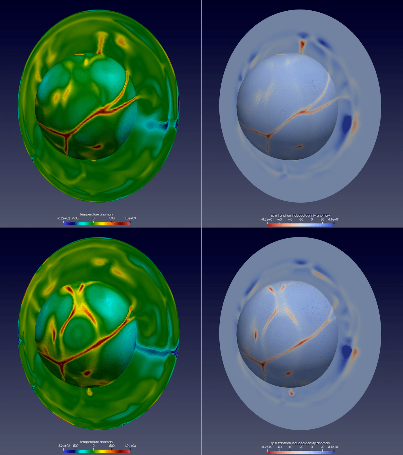
Figure 2: Temperature anomaly (left) and the corresponding spin transition-induced density anomaly (right) at two timesteps separated by 20 Myrs (earlier at the top) in a cross-section and at the inner, core-mantle boundary. You can see a descending cold slab that becomes first lighter and then heavier (red and blue regions on the right panels) which can initially slow and then accelerate the mantle flow at mid-mantle depths (bottom left panel). You can see similar effects in the hot rising plumes. These two effects can cause plume or slab stagnation at mid-mantle depths with subsequent sudden avalanches.